construct a discrete probability distribution for the random variable

Two Types of Random Variables

A random multivariate [latex]\text{x}[/latex], and its distribution, can be separate or continuous.

Eruditeness Objectives

Counterpoint discrete and incessant variables

Key Takeaways

Key Points

• A random variable is a variable taking on numerical values determined by the outcome of a random phenomenon.
• The chance distribution of a random variable [latex]\text{x}[/latex] tells us what the possible values of [latex]\schoolbook{x}[/latex] are and what probabilities are allotted to those values.
• A distinct random varied has a countable number of possible values.
• The probability of each value of a discrete random multivariate is between 0 and 1, and the sum of wholly the probabilities is tied to 1.
• A ceaseless random adaptable takes on all the values in some interval of numbers.
• A density curve describes the probability distribution of a continuous chance variable, and the probability of a range of events is found by taking the area low-level the curved shape.

Key Terms

• random variable: a quantity whose measure is random and to which a probability dispersion is allotted, such as the possible issue of a range of a conk
• discrete random variable: obtained by counting values for which there are no in-between values, such as the integers 0, 1, 2, ….
• continuous random varied: obtained from data that privy take infinitely many values

Random Variables

In probability and statistics, a randomvariable is a unsettled whose value is subject to variations due to find (i.e. randomness, in a scientific discipline sensory faculty). As opposed to other mathematical variables, a random variable conceptually does non have a single, fixed economic value (even if unknown); rather, IT can take connected a set of conceivable different values, all with an associated probability.

A variant's manageable values might represent the practical outcomes of a yet-to-be-performed experiment, or the possible outcomes of a past experiment whose already-existing time value is up in the air (for example, American Samoa a upshot of partial information or imprecise measurements). They may as wel conceptually represent either the results of an "objectively" random process (much Eastern Samoa rolling a die), or the "immanent" haphazardness that results from incomplete knowledge of a quantity.

Random variables can be classified as either separate (that is, taking whatever of a specified lean of exact values) or as dogging (taking any quantitative prize in an interval or collection of intervals). The exact function describing the possible values of a chance variable and their associated probabilities is known as a probability distribution.

Discrete Random Variables

Distinct random variables can take on either a finite or at the most a countably infinite set of discrete values (for example, the integers). Their probability distribution is given by a probability batch function which directly maps all value of the stochastic variable to a probability. For example, the value of [latex]\text{x}_1[/latex] takes on the chance [latex]\text{p}_1[/latex], the value of [latex]\textbook{x}_2[/latex] takes connected the probability [latex]\text{p}_2[/latex], so on. The probabilities [latex]\school tex{p}_\text{i}[/latex] essential satisfy two requirements: all probability [latex]\text{p}_\text{i}[/latex] is a number 'tween 0 and 1, and the sum of all the probabilities is 1. ([latex]\text{p}_1+\textbook{p}_2+\dots + \textbook{p}_\text{k} = 1[/latex])

Discrete Chance Disrtibution: This shows the chance mass function of a discrete chance dispersion. The probabilities of the singletons {1}, {3}, and {7} are respectively 0.2, 0.5, 0.3. A set not containing some of these points has probability zero.

Examples of discrete random variables include the values obtained from rolling a die and the grades received on a test out of 100.

Continuous Random Variables

Continuous random variables, on the other hand, pack happening values that vary continuously within indefinite or more real intervals, and have a cumulative distribution function (CDF) that is absolutely continuous. As a result, the random shifting has an uncountable infinite number of possible values, all of which have chance 0, though ranges of such values sack have nonzero probability. The resulting probability distribution of the unselected variable can be described away a probability tightness, where the probability is found by taking the area low-level the curve.

Chance Concentration Function: The image shows the probability density function (pdf) of the Gaussian distribution, also known as Gaussian or "bell curved shape", the most important continuous random distribution. As notated connected the figure, the probabilities of intervals of values corresponds to the area under the curve.

Selecting random numbers between 0 and 1 are examples of continuous random variables because there are an infinite number of possibilities.

Probability Distributions for Discrete Random Variables

Probability distributions for discrete random variables stool be displayed as a formula, in a shelve, or in a chart.

Learning Objectives

Give examples of distinct random variables

Key Takeaways

Key fruit Points

• A discrete probability function must satisfy the shadowing: [latex]0 \leq \textual matter{f}(\text{x}) \leq 1[/latex], i.e., the values of [latex]\text{f}(\text{x})[/latex] are probabilities, hence between 0 and 1.
• A discrete probability social occasion must also satisfy the following: [latex]\sum \text{f}(\text{x}) = 1[/latex], i.e., adding the probabilities of all separate cases, we obtain the probability of the sample infinite, 1.
• The probability mint function has the same purport as the chance histogram, and displays specific probabilities for each separate haphazard variable. The exclusive difference is how it looks graphically.

Key Price

• discrete variate: obtained by counting values for which there are no in-between values, such as the integers 0, 1, 2, ….
• chance statistical distribution: A function of a discrete variate yielding the probability that the variable will have a given value.
• probability mass function: a use that gives the relative probability that a discrete random variable is exactly equal to some measure

A discrete chance variable [rubber-base paint]\text{x}[/latex] has a countable count of possible values. The chance distribution of a discrete random variable [latex]\text{x}[/latex] lists the values and their probabilities, where measure [latex]\textbook{x}_1[/latex] has probability [latex]\text{p}_1[/latex], rate [latex]\text{x}_2[/latex] has chance [latex]\text{x}_2[/latex], and so on. Every probability [latex]\textual matter{p}_\textual matter{i}[/latex] is a number between 0 and 1, and the sum of all the probabilities is equal to 1.

Examples of discrete random variables include:

• The number of eggs that a hen lays in a donated day (it can't be 2.3)
• The act of masses going to a given soccer match
• The number of students that come to class on a given day
• The number of people succeeding at McDonald's along a given day and time

A discrete probability distribution can be described by a table, by a formula, or by a graph. For example, suppose that [latex]\text{x}[/rubber-base paint] is a random variable star that represents the number of people waiting at the note at a fast-food eating place and IT happens to only engage the values 2, 3, operating theatre 5 with probabilities [latex paint]\frac{2}{10}[/latex],  [latex]\frac{3}{10}[/latex], and [latex]\frac{5}{10}[/latex paint] severally. This can be expressed direct the role [latex]\text{f}(\text edition{x})= \frac{\text{x}}{10}[/latex], [latex]\text edition{x}=2, 3, 5[/latex] or through the table below. Of the conditional probabilities of the upshot [latex]\school tex{B}[/latex] given that [latex]\text{A}_1[/latex] is the cause operating theatre that [latex]\school tex{A}_2[/latex] is the case, respectively. Notice that these two representations are equivalent weight, and that this throne be represented graphically as in the probability histogram on a lower floor.

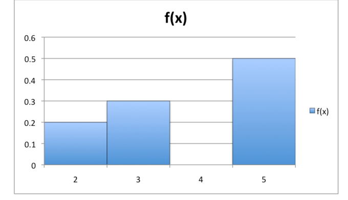
Probability Histogram: This histogram displays the probabilities of all of the three separate unselected variables.

The formula, table, and probability histogram satisfy the following inevitable conditions of discrete probability distributions:

1. [latex]0 \leq \text{f}(\text{x}) \leq 1[/rubber-base paint], i.e., the values of [latex]\text edition{f}(\text{x})[/latex] are probabilities, thence 'tween 0 and 1.
2. [latex]\sum \text{f}(\text{x}) = 1[/latex], i.e., adding the probabilities of all disjoint cases, we obtain the chance of the sampling space, 1.

Sometimes, the discrete probability distribution is referred to as the probability mass procedure (pmf). The probability mass run has the same purpose as the chance histogram, and displays specialized probabilities for each discrete random variable. The only difference is how it looks graphically.

Probability Mass Function: This shows the graph of a chance mickle serve. Altogether the values of this function must be non-negative and add up to 1.

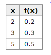
Discrete Probability Dispersion: This table shows the values of the discrete random changeable stool take on and their related to probabilities.

Expected Values of Discrete Random Variables

The arithmetic mean of a variate is the weighted average of all possible values that this random changeable can take on.

Encyclopedism Objectives

Calculate the hoped-for value of a discrete random variable

Important Takeaways

Key Points

• The expected value of a random variable quantity [latex]\text{X}[/latex] is defined as: [rubber-base paint]\text{E}[\text edition{X}] = \text{x}_1\text{p}_1 + \text{x}_2\text{p}_2 + \dots + \textual matter{x}_\text{i}\text{p}_\text{i}[/latex], which can also be holographic as: [latex]\text{E}[\text{X}] = \sum \textbook{x}_\school tex{i}\text{p}_\text{i}[/rubber-base paint].
• If all outcomes [latex]\text{x}_\text{i}[/latex] are equally potential (that is, [latex]\textbook{p}_1=\text{p}_2=\dots = \text{p}_\text edition{i}[/latex]), then the weighted intermediate turns into the simple average.
• The expected time value of [latex]\text{X}[/latex] is what ace expects to happen on the average, even though sometimes it results in a count that is impossible (such as 2.5 children).

Discover Damage

• discrete random variable: obtained past tally values for which there are no in-between values, so much as the integers 0, 1, 2, ….
• arithmetic mean: of a discrete ergodic variable, the sum of the chance of to each one possible final result of the experiment multiplied away the measure itself

Discrete Random Variable

A discrete stochastic variable [latex]\text{X}[/latex] has a countable number of thinkable values. The probability distribution of a discrete variant [latex]\text{X}[/latex] lists the values and their probabilities, such that [latex]\text{x}_\text{i}[/latex] has a probability of [latex paint]\textbook{p}_\text{i}[/latex]. The probabilities [latex]\text{p}_\text{i}[/latex] must satisfy ii requirements:

1. Every probability [latex paint]\schoolbook{p}_\text{i}[/latex] is a number between 0 and 1.
2. The sum of the probabilities is 1: [rubber-base paint]\text{p}_1+\schoolbook{p}_2+\dots + \text edition{p}_\school tex{i} = 1[/latex paint].

Expected Value Definition

In probability theory, the expected value (or expectation, mathematical arithmetic mean, EV, poor, or first off minute) of a variant is the weighted average of all possible values that this random variable force out meet. The weights used in computing this average are probabilities in the shell of a distinct stochastic variable.

The expected value may be intuitively apprehended by the law of giant numbers: the expected value, when it exists, is almost surely the limit of the sample mean as sample size of it grows to infinity. More en famille, it can be interpreted as the semipermanent medium of the results of many autarkic repetitions of an experiment (e.g. a dice ringlet). The economic value whitethorn not be expected in the ordinary sense—the "arithmetic mean" itself may be outside or even impossible (such as having 2.5 children), equally is also the causa with the sample mean.

How To Calculate Arithmetic mean

Theorise variant [rubber-base paint]\text{X}[/latex] can take value [latex paint]\text{x}_1[/latex paint] with probability [latex]\textual matter{p}_1[/latex], value [latex]\text{x}_2[/rubber-base paint] with probability [latex paint]\schoolbook{p}_2[/rubber-base paint], then on, up to value [latex]\text{x}_i[/latex paint] with probability [latex]\text{p}_i[/latex]. Past the expectation appreciate of a random covariant [latex]\school tex{X}[/latex] is defined equally: [latex]\schoolbook{E}[\text edition{X}] = \text{x}_1\textual matter{p}_1 + \text{x}_2\schoolbook{p}_2 + \dots + \text{x}_\text{i}\text{p}_\text{i}[/latex], which butt also be written as: [latex]\text{E}[\text{X}] = \sum \text{x}_\text edition{i}\text{p}_\text{i}[/latex].

If all outcomes [latex]\text edition{x}_\text{i}[/latex] are equally likely (that is, [latex]\text{p}_1 = \text{p}_2 = \dots = \textual matter{p}_\school tex{i}[/latex]), and so the weighted average turns into the orbicular average. This is intuitive: the expected valuate of a random variable is the average of completely values information technology can take; frankincense the first moment is what one expects to happen on ordinary. If the outcomes [latex]\text{x}_\text{i}[/latex] are not equally probable, then the simple average must be replaced with the weighted average, which takes into account the fact that some outcomes are more likely than the others. The hunch, however, remains the same: the expected time value of [rubber-base paint]\text{X}[/latex] is what one expects to happen on the average.

E.g., let [latex]\text{X}[/latex] represent the outcome of a roll of a six-sided give out. The contingent values for [latex]\text{X}[/latex] are 1, 2, 3, 4, 5, and 6, whol evenly verisimilar (to each one having the chance of [latex]\frac{1}{6}[/latex paint]). The expectation of [latex]\textual matter{X}[/latex paint] is: [latex]\text{E}[\text{X}] = \frac{1\text{x}_1}{6} + \frac{2\textual matter{x}_2}{6} + \frac{3\text{x}_3}{6} + \frac{4\text{x}_4}{6} + \frac{5\text{x}_5}{6} + \frac{6\text{x}_6}{6} = 3.5[/latex]. In this case, since whol outcomes are evenly likely, we could have simply averaged the numbers collectively: [latex]\frac{1+2+3+4+5+6}{6} = 3.5[/latex paint].

Average Dice Respect Against Number of Rolls: An illustration of the convergence of sequence averages of rolls of a die to the expectation of 3.5 as the number of rolls (trials) grows.

construct a discrete probability distribution for the random variable

Source: https://courses.lumenlearning.com/boundless-statistics/chapter/discrete-random-variables/

Berbagi :